Ground Reflections

Summary

Paths with ground reflections

Reflection coefficient

Received signal level

Diversity reception

Performance degradation

HERALD Lab #4

_______________________________________________________________

Summary

A radio path with ground reflection is examined. The reflection coefficient of different surfaces is discussed and several examples are given. The loss in received signal power is estimated, including the effect of antenna positioning and k-factor. Finally, the use of space diversity is considered and overall degradation is evaluated.

Paths with ground reflection

In radio hops over flat surfaces and particularly over the sea (or other large water surfaces), a fraction of the EM power emitted by the transmitter may reach the Rx antenna after reflection on the flat surface. So, at the receiver, the direct signal and the reflected signal (both coming from the same transmitter) may interfere each other.

Signal reflections represent in most cases a critical aspect of radio hop design and a potential source of operating problems, if not correctly evaluated at the design stage.

In route planning and site selection, a priority objective should always be to avoid hops with possible ground reflections, as far as possible. Obviously, alternative routes may be possible only in limited cases.

A careful selection of site positioning and antenna height may be of help in situations where such solution makes the reflected ray obstructed, at least partially. While discussing on received signal level, it will be shown that any technique, that reduces in some measure the reflected signal level, is useful in reducing the overall impact of signal reflection.

The first step in reflection analysis is to get all the geometrical elements useful to describe the reflection mechanism. The figure below gives a sketch of a radio path with ground reflection, showing the main geometrical parameters.

Path with ground reflection, main geometrical parameters.

· P = Reflection point;

· g = Grazing angle;

· D = Direct path length;

· R1+R2 = Reflected path length;

· DL = R1+R2 - D = path length difference;

· a1, a2 = Angles between Direct and Reflected rays at the two antennas.

Reflection coefficient

By comparing the reflected radio wave to the incident one, amplitude and phase modifications are observed. The reflection coefficient is a complex number, where :

· the coefficient modulus is the amplitude ratio between the reflected and the incident signals; it represents the signal attenuation due to the reflection effect only;

· the coefficient phase gives the phase shift produced by reflection (phase difference between the reflected and the incident signals).

The reflection coefficient is a function of :

· signal frequency and polarization;

· grazing angle g;

· electrical parameters of the reflecting surface (relative permittivity and conductivity; diagrams are given in ITU-R Rec. P-527 for different surface types: water, dry soil, wet soil, etc.).

Additional attenuation is caused by surface roughness, depending on soil irregularities or sea waves. However, smooth surface parameters usually represent a worst case assumption, with minimum loss.

Summary of results

At very low grazing angles (g < 0.2 deg), the reflection coefficient amplitude, on sea surfaces or wet soil, is close to unity (0 dB) for both vertical and horizontal polarization; the phase is close to 180 deg.

For horizontal polarization (any frequency), the above results are almost unchanged when g increases up to about 4 deg (higher values of the grazing angle are very unlikely).

On the other hand, with vertical polarization and the same range of the grazing angle, the reflection coefficient amplitude decreases to about 0.3 - 0.5 (-10 to -6 dB, the lowest loss being applicable to frequencies above 10 GHz). Also the phase decreases to 120° - 140° for frequencies in the 1 - 3 GHz range, while it is closer to 180° range for frequencies above 10 GHz.

While the above results only give approximate indications on the actual numbers to use in path design, it must be realized that the variable environment (for example, wet or dry soil) and the surface roughness make it difficult even to apply specific models and formulas to predict the reflection coefficient.

In most cases, it is advisable to make use of worst case assumptions for the coefficient amplitude, while not always a precise prediction on the phase shift is required (as explained below).

Reflection coefficient computation

For a plane surface, the reflection coefficient G can be computed, according to the Fresnel law, as :

Vertical polarization

Horizontal polarization.

where

is called complex permittivity, g is the grazing angle, l [m] is the signal wavelength, while the electrical parameters of the reflecting surface are :

e_r relative dielectric constant;

s electrical conductivity.

The expressions giving the reflection coefficient G can be specialized to the most common reflecting surfaces, taking account of typical values of the surface electrical parameters at different frequencies, as shown in the Tables below.

Relative dielectric constant e_r (dimensionless parameter) :

1 GHz

3 GHz

10 GHz

30 GHz

Sea water

Fresh water

Wet ground

5.4

Very dry ground

Ice (-1 -10 °C)

Electrical conductivity s [ohm^-1 m^-1] :

1 GHz

3 GHz

10 GHz

30 GHz

Sea water

Fresh water

0.18

1.8

Wet ground

0.15

0.7

3.2

Very dry ground

1.5 10^-4

0.003

0.05

0.35

Ice (-1 -10 °C)

2.5 - 8 10^-4

0.6 - 2 10^-3

2 - 6

10^-3

0.5 - 1.7 10^-2

Example of results are shown in the figures below.

Reflection over the sea surface

Amplitude of the reflection coefficient vs. grazing angle.

Reflection over the sea surface

Phase of the reflection coefficient vs. grazing angle.

Reflection over a fresh water surface

Amplitude of the reflection coefficient vs. grazing angle.

Reflection over a fresh water surface

Phase of the reflection coefficient vs. grazing angle.

Reflection over very dry soil

Amplitude of the reflection coefficient vs. grazing angle

(the phase is close to 180° for both H and V polarization).

Received signal level

The Rx signal power results from the addition of the Direct and the Reflected signals

Vectorial addition of two signals

We measure "relative" signal amplitude and power as referred to the direct signal only. The Relative Rx Power (RRP, in dB), in the presence of a reflected ray, is :

where b, b are the relative amplitude and phase of the reflected ray, at the receiver input. The relative power (B, in dB) of the reflected signal is :

The figure below gives some examples of the result of the vectorial addition of two signals, with different amplitudes and varying relative phase.

Received signal power in the presence of a reflected signal,

whose relative power B is indicated by the labels

(relative power is referred to the direct signal alone).

As expected, if the direct and the reflected signals have equal amplitude (0 dB curve), then the resulting signal fades completely when the two signals are in phase opposition (relative phase 180 deg). On the other hand, if the reflected signal is more and more attenuated (B = -10, -20 dB curves), then the overall Rx signal shows a moderate fluctuation, as a function of the relative phase between the direct and the reflected signals.

Reflected signal amplitude

In order to estimate the relative amplitude of the two signals, we have to identify the additional attenuation in the reflected signal, compared to the direct one. Additional attenuation is mainly caused by :

· Reflection coefficient: as discussed above, it depends on signal frequency and polarization, grazing angle and surface electrical parameters; for reflection over water, the 0 dB loss (perfectly reflecting surface) may be a worst case assumption.

· Divergence factor: this is a geometrical factor, which accounts for the spherical shape of the reflecting earth surface, producing a divergence in the reflected beam (not negligible in reflection paths with very small grazing angle).

· Antenna gain reduction: assuming that the antenna is pointed in the direct ray direction, then the gain in the reflected ray direction is given by the antenna diagram at angles a1 and a2 (see reflection geometry); quite often these angles are very small, but in some cases (e.g. short hops with antennas very high over the reflecting surface) they produce a not negligible reduction in the antenna gain. Even in absence of the complete antenna diagram, the 3dB antenna beamwidth in the vertical plane can be sufficient to estimate the reduction in antenna gain for a small deviation from the antenna axis.

· Obstruction loss (if the reflection path is not perfectly clear): in most cases it can be estimated as a "knife edge" obstruction, because this is a conservative assumption and it is usually close to the actual conditions.

Reflected signal phase

On the other hand, the phase shift between the direct and the reflected signals depends on :

· Path length difference DL: this distance is converted into a phase shift, taking into account that a signal wavelength l corresponds to a 360 deg phase rotation :

· Reflection coefficient phase: as discussed above, in most cases it is close to 180 deg (phase reversal).

Rate of change in the Rx signal amplitude

Since the wavelength l is of the order of centimeters, then in most cases DL >> l. In such conditions, the above formula shows that a fractional change in DL (as caused even by small k-factor variations) produces a significant rotation of the d phase. The final effect is that :

· the direct and the reflected signals add with a variable phase shift, which can be assumed as a random variable; amplitude fluctuations are to be expected in the sum signal (received signal);

· the reflection coefficient phase is not so important to be predicted, since it adds to the (randomly) variable phase shift d;

On the other hand, when DL is of the same order of magnitude of (or even smaller than) l, a fractional change in DL produces a small rotation of the d phase. So, in the vectorial addition of the direct and reflected signals, the phase angle is almost constant and slow variations in the Rx power level are likely (low levels may persist for long periods of time).

Antenna height and k-factor effect

The above discussion shows that the reflected signal amplitude and phase (relative to the direct one) are functions of the geometrical reflection parameters. So, we expect that

· the overall Rx signal level is a function of antenna position;

· for a given antenna position, the Rx signal level is time variable, due to atmospheric variations (changing k-factor);

· in particular cases, a time-variable Rx level may be also produced by variations in the reflecting surface (for example, tide movements).

The figure below (continuous line) shows the Rx power level vs. antenna position. For a given antenna height (H1) the two signals (direct and reflected) add in phase, so that the Rx signal level is maximum, while for a different antenna position (H2) the two signals are in phase opposition and the Rx level is minimum.

Received signal power vs. antenna height,

with two values of the k-factor (continuous and dashed lines) (relative power is referred to the direct signal alone).

The dashed line refers to a different atmosphere condition (different k-factor) and shows that, even if the plots are similar, the antenna positions corresponding to max / min Rx signal power are not stable.

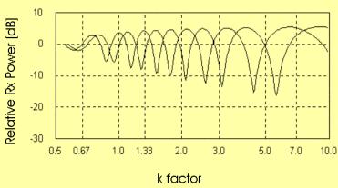
The effect of varying atmospheric conditions (k-factor) is presented in the figure below. At a constant antenna height, the received signal level may be at a maximum or minimum value, depending on variations in the k-factor.

Received signal power vs. k-factor, for a given antenna height

(relative power is referred to the direct signal alone).

Note : The examples given in the previous figures are for a given reflection geometry, working frequency, etc. Other patterns in the Rx power diagrams may be found with different parameters. However, the comments suggested by these figures hold in most applications.

In summary :

· we cannot predict the exact antenna position corresponding to maximum or minimum Rx power levels (since this is not a static conditions, due to k-factor variations);

· we can however compute the Rx power range (vs. antenna position and k-factor);

· we can also compute the vertical distance (H2 - H1) between the antenna position for maximum Rx power and minimum Rx power.

Diversity reception

Generally speaking, we implement a diversity system by using two different communications channels to transmit the same information. At the receiver, the signals at the output of the two channels are processed to get a reliable estimate of the transmitted information. Basically, two techniques can be used :

· the selection of the signal that, at a given time, is estimated to offer the best quality (diversity switching);

· the joint processing of the two signals (diversity combining).

A number of alternative implementations have been studied for each of the above techniques, taking account of different operating contexts and design constraints.

In any case, the basic requirement for effective diversity systems is that of a low correlation between the two channels, so that a low probability exists that both channels are in a bad state at the same time.

In radio paths with ground reflection, the two different communications channels can be implemented by using two vertically separated antennas at the receiver site (space diversity).

The reflection geometry is different for the two channels (different reflection point P1 and P2, see figure below). So, it is expected that different signal levels are received at the two antennas, at a given time.

Space Diversity reception in a radio hop with ground reflection

In order to find the optimum vertical spacing between the two antennas, we compute the spacing DH = (H2 - H1) between a maximum and a minimum in the Rx power vs. antenna height diagram.

With antenna spacing DH, it is expected that, while the Rx power level is minimum at one antenna, it is close to the maximum at the other antenna, and vice versa. So, both antennas are never in bad reception at the same time.

This estimate of the optimum spacing applies to a given k-factor value. As a first guess, the DH spacing is computed with the standard k value (1.33). Depending on the reflection geometry, this choice may be appropriate (or not) also for different k values.

The figure below shows the Rx power at the two antennas vs. k-factor. It gives a simple way to check how the antenna spacing, computed for a given k, works with other k values.

Same figure as above, with a diversity antenna added;

optimum diversity spacing computed for k = 1.33

(relative power is referred to the direct signal alone).

In this example, we see that at least one of the two antennas receives a high power level for any k value greater than 1 (the max/min patterns of the two diagrams are well interleaved). On the other hand, going to low k values (k<1), the two diagrams are closer and almost overlapping, so the diversity effect vanishes.

If the antenna spacing, optimized for standard k-factor, is not effective for other k-factors, possible suggestions are :

· to find a compromise solution, taking account of the likely range of k-factor values;

· to revise (if possible) the overall reflection geometry (for example, by modifying the antenna height also at the other hop terminal).

In implementing a space diversity configuration, usually the additional (diversity) antenna is installed below the main antenna. The clearance rules for the main antenna are as indicated in the Path Clearance session.

For the diversity antenna, ITU-R Rec. P-530 gives the following clearance criteria :

· Normalized clearance C_NORM > 0.3 for an isolated obstacle;

· Normalized clearance C_NORM > 0.6 for an obstacle extended along a portion of the path.

The above limits may be reduced to 0.0 and 0.3, respectively, "if necessary to avoid increasing heights of existing towers" and if the frequency is below 2 GHz.

Performance degradation

In the previous chapters, the received signal power has been estimated for single and diversity reception, as a function of antenna positioning and atmospheric state (k-factor).

Under some aspects, it is necessary to make worst case assumptions, for example in the estimate of the reflection coefficient.

An overall estimate of performance degradation caused by ground reflection requires that the Rx power loss be averaged over the whole range of operating conditions.

The average loss in Rx signal power is estimated for a given k-factor, by assuming the phase shift between the direct and the reflected signals as a random variable. Moreover, it is possible to further average, over the expected range of k-factor variations.

Note that the signal phase shift can be assumed as a random variable only if DL >> l (path difference much larger than wavelength); this assumption has been discussed previously.

When diversity reception is adopted, a similar average can be performed but, for each operating conditions (k-factor value, signal phase shift), the antenna with the higher signal is selected. This is equivalent to a diversity system with ideal and instantaneous switching to the best signal; therefore, the results computed under the above assumptions may be optimistic in some measure.

Average degradation estimate

The Rx signal power loss (LOSS_REFL), in the presence of a reflected ray, is given by the ratio of the direct signal power (normalized to 1) to the Rx power with reflection :

where b, b are the relative amplitude and phase of the reflected ray, at the receiver input.

When, for a given reflection geometry and atmospheric state (k-factor), we can assume b as a random variable (see comments on the rate of change in the Rx signal amplitude), then the LOSS_REFL average over the b uniform distribution is given by (the bar over a symbol means "average value") :

(the integral solution is not immediate and requires some careful mathematical processing).

Finally, the Threshold Degradation due to reflection D_REF (in dB) is given by :

In more general terms, it also necessary to further average the Rx signal power loss LOSS_REFL, over a range of likely k-factor values, since the reflection geometry (and specifically the reflected ray amplitude b) is a function of k. Then we need to estimate an integral expression of the type :

This is usually possible only by numeric integration methods.

In digital radio systems, additional degradation may be caused by signal distortions, when the time delay of the reflected signal is comparable with the symbol period of the digital modulation. This is not a usual condition, but it is to be considered with some care.

Effect of time delay on digital signals

In digital radio links, it is necessary to compare the reflected signal delay t with the symbol period T_S, in order to estimate the reflection impairment on the digital modulation.

When t << T_S there is no significant distortion of the digital signal format, since the modulated pulses in the direct and reflected signals are almost overlapping at the receiver; the only reflection impairment is due to the Rx signal attenuation, as discussed previously.

If t is comparable (<=) with T_S, then the two-path (direct plus reflected signals) channel transfer function produces a frequency-selective distortion on the signal spectrum. The equipment signature gives a measure of the additional reflection impairment, due to Rx sensitivity to signal distortion.

Finally, the condition t > T_S is very unlikely. However, in this case, the reflected signal appears as an external co-channel interference, since the modulation applied to the direct signal is not coincident with the modulation in the reflected signal. The equipment BER vs. C/I curve gives a measure of performance degradation under this condition.