Path
Clearance
![]() Refractivity
in the Atmosphere
Refractivity
in the Atmosphere
![]() Propagation
in Standard Atmosphere
Propagation
in Standard Atmosphere
© 2001-2014,
Luigi Moreno, Torino, Italy
_______________________________________________________________
Summary
In this Session the
effect of the atmosphere on radio ray trajectories is first considered, by
introducing the k-factor concept; possible deviations from standard conditions
are identified, as well as the minimum k-factor value. Then the Fresnel
ellipsoid is defined; the partial obstruction of the ellipsoid leads to the
estimate of the resultant loss. Finally, the previous concepts are used to set
clearance criteria and to discuss their application to path profile analysis.
Refractivity
in the Atmosphere
The Refractive Index n in a given medium is
defined as the ratio of the speed of radio waves in vacuum to the speed in that
medium. Since the speed of radio waves in the atmosphere is just slightly lower
than in vacuum, then the Refractive Index in the atmosphere is greater than,
but very close to, 1.
However, also
small variations in the atmosphere Refractive Index have significant effects on
radio wave propagation. For this reason, instead of using the Refractive Index
n (close to 1), it is convenient to define the Refractivity N as :
![]()
So, N is the
number of parts per million that the Refractive Index exceeds unity; it is a
dimensionless parameter, measured in N-units.
The atmosphere
Refractivity is a function of Temperature, Pressure, and Humidity. The ITU-R
Rec. 453 gives the formula :
where :
T = absolute temperature (Kelvin deg);
P = atmospheric pressure (hPa, numerically equal to millibar);
e = water vapour pressure (hPa).
At sea level, the
average value of N is about No = 315 N-units. The ITU-R gives world maps with
the mean values of No in the months of February and August.
Temperature, atmospheric pressure, and water vapour pressure are not
constant with height. This produces a Vertical Refractivity Gradient G
(measured in N-units per km, N/km), defined as:
where N1
and N2 are the refractivity values at elevations H1 and H2,
respectively.
Under normal
(standard) atmospheric conditions,
Refractivity decreases at a constant rate, moving from ground level up
to about 1 km height. This means that
the Refractivity Gradient G is constant, the typical value being about -40
N/km.
Deviation from the
Standard Atmosphere condition is usually associated with particular weather
events, like temperature inversion, very high evaporation and humidity, passage
of cold air over warm surfaces or vice versa. In these conditions, the Vertical
Refractivity Gradient is no longer constant. A number of different profiles
have been observed and measured. It is worth noting that, at greater altitude, the
Refractive Index is, in any case, closer and closer to 1; so the Refractivity N
decreases to zero.
Propagation in Standard
Atmosphere
A Radio Wave propagates in the direction
normal to the iso-phase plane (the plane where all the points are phase
synchronous, with respect to the sinusoidal pattern of electric and magnetic
fields).
In a homogeneous
medium, the iso-phase planes are parallel to each other and the propagation
direction is a straight line normal to them.
As seen above, the Atmosphere is not a
homogeneous medium and the Vertical Refractivity Gradient gives a measure of that.
Different Refractivity at different heights means different propagation speeds.
The wave-front moves faster or slower, depending on the height: this causes a
rotation of the wave-front itself.
Wave-front and ray rotation
caused by a vertical
refractivity gradient in the atmosphere
So, the
propagation trajectory (normal to the wave-front) is not a straight line, but
it is rotated, as shown in the above figure. Taking into account that the
propagation speed is inversely proportional to the refractive index, it is
possible to derive that the radio trajectory curvature
1/r is related to the Vertical Refractivity Gradient G, as :

In Standard
Atmosphere, with a typical value of the Refractivity Gradient G = -40 N/km, the curvature of the radio ray
trajectory is :
This means that
the radio ray is bent downward, with a curvature 1/r, somewhat lower (less
curved) than the Earth curvature 1/R :

Ray bending in standard atmosphere
(CL = clearance, vertical distance from ground to ray trajectory)
The k-factor
A convenient artifice is used to account, at the same
time, for both the ray and the earth curvatures. An "equivalent"
representation of the above figure
can be plotted by altering both curvatures by an amount equal to the ray
curvature 1/r.
In
the new figure (see below) the radio ray trajectory becomes a straight line,
while the modified ("equivalent") earth curvature 1/RE is
:
Equivalent representation of the
previous figure,
with a modified earth radius RE and a straight ray
trajectory.
Note that, at any
point of the radio path, the vertical distance (CL = clearance) from the earth
surface to the ray trajectory is the same in the real and in the equivalent
representations.
The ratio between the
equivalent and the real earth radius is defined as the "effective
earth-radius factor k" (briefly, the k-factor). Taking account of previous formulas, giving 1/RE, 1/R, and 1/r
, the k-factor is given by :
In Standard
Atmosphere (G = -40 N units/km), this gives :
![]()
The k-factor gives
an indication about the atmosphere state at a given time and about the bending
effect on the radio ray trajectory. So, the statement "propagation at k =
4/3" is a synonymous of "propagation in Standard Atmosphere".
On the other hand, k < 4/3 corresponds to "Sub-refractive"
conditions, in which the ray curvature is
less than normal or even is an
upward curvature ( k < 1, G > 0 ), thus
reducing the clearance over ground.
With k > 4/3 we
are in a "Super-refractive" atmosphere; in particular, with k = ¥, the ray trajectory is parallel to the earth
surface and the signal can propagate over
large distances, beyond the normal horizon.
The figure below
compares the ray trajectories with different k-factors, using a "real
earth" representation.
Ray bending in different atmospheric conditions
(different k-factor values)
A further
alternative in plotting radio ray trajectories over the earth surface, is
called "flat earth" representation
Again, both the
earth and the ray curvature are altered, but in this case the earth profile is
forced to be flat, while the ray curvature is modified accordingly. The
"real earth" and the "flat earth" diagrams are equivalent
in the sense that, at any point
of the radio path, the vertical distance (CL = clearance) from the earth
surface to the ray trajectory is the same in both representations.
Equivalent representation of the previous figure, over flat earth
Using the
"flat earth" representation, we can plot on the same diagram the path
profile and multiple rays, corresponding to different values of the
k-factor. This is the most usual diagram
shown in computer applications for radio hop design.
k-Factor variability
We have seen that the k-factor is related to
the atmosphere state and is a function of the refractivity vertical gradient.
So, it is a variable parameter, depending
on daily and seasonal cycles and on current
meteorological conditions. In a "standard atmosphere" state
the k-factor value is 4/3; this is close to the median value in most climates
(particularly, temperate climates). Around this median value, the range of variations is rather wide in
tropical regions, with increasing temperature and/or humidity, while it is more
limited in cold and temperate climates.
Experimental
observations show for example that the probability of k<0.6 in temperate
climates is generally well below 1%. In tropical climates the same event is
observed with probability in the range 5% - 10%. This means that, in tropical
regions, there is the highest probability of propagation anomalies due to
extreme k-factor values. The ITU-R gives world maps of the time percentage with
G < -100 N-units / km (k > 2.75), in different months.
In discussing
k-factor variability, as applied to radio hop design and to clearance criteria,
we have to consider that:
· In sub-refractive conditions
(minimum k-factor) the clearance over
ground is reduced and the
probability of obstruction is maximum.
· We
are not interested in the minimum "local" k-factor, but in the
overall effect through the whole radio path. So an "equivalent
k-factor" (kea) is defined, whose minimum value depends (for given climatic conditions) on the path length.
On long hops kea is
likely to be not far from standard values, because extreme atmosphere
conditions are probably not present at a time on the whole path, while in
shorter hops it is more likely that particular events affect almost the whole
path and produce lower kea values.
The ITU-R (Rec. P-530) gives a curve of minimum kea values as a function of hop length (temperate climate).
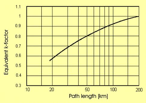
Minimum equivalent k-factor vs. path length
(from ITU-R Rec. P-530, by IT permission).
Fresnel Ellipsoid
From a geometrical point of view, the Fresnel
ellipsoid is defined as the set of points (P) in the space which satisfy the
equation :
![]()
where Tx and Rx are the two antennas (radio
path terminal points), representing the two focuses of the ellipsoid.
The Fresnel ellipsoid, F1 = ellipsoid radius;
CL = clearance, measured from earth surface to the ray trajectory (that
is the ellipsoid longitudinal axis)
The radioelectrical interpretation of the
Fresnel ellipsoid is that two rays, following the paths Tx-Rx and Tx-P-Rx,
arrive at the Rx antenna in phase opposition (half-wavelength path difference,
then 180 deg phase shift).
The Fresnel ellipsoid radius F1 (in meters), at a distance D1 from one
of the radio sites, is given by :
where D (km) is
the path length, F (GHz) is the frequency and l (m)
is the wavelength. Some examples are
given in the figure below; note that the Fresnel ellipsoid radius reduces as
frequency increases.
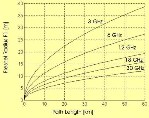
Fresnel ellipsoid radius vs. path length and frequency
(max radius, computed at mid
path length).
From a practical
point of view, the Fresnel ellipsoid gives a rough measure of the space volume involved
in the propagation of a radiowave from a source (Tx) to a sensor (Rx). About
half of the Rx signal energy travels through the Fresnel ellipsoid. So, any
obstruction within the Fresnel ellipsoid has some impact on the Rx power level.
This leads to
consider radio visibility in terms of clearance of the Fresnel ellipsoid, as
discussed below.
![]()
A note on radio
propagation and visual analogies
We are
familiar with our visual experience and this can be of help in describing some
aspects of radio propagation.
However, the
Fresnel ellipsoid shows that radio propagation (like any EM propagation effect)
cannot be explained only in terms of geometric optics, that is adequate so long as any discontinuities
encountered through the propagation path are very large compared with the
wavelength.
The ellipsoid radius is proportional to
the wavelength square root. In our visual experience, the light wavelength is
so small (about 5 10-4 mm) that the radius of the Fresnel ellipsoid
is negligible, at least as a first approximation. Diffraction effects can be
observed only with accurate experiments, showing the role of Fresnel ellipsoid
also in the optical field.
On the other
hand, in radio communications the wavelength is in the range from 1 m
(frequency 300 MHz) to about 1 cm (frequency 30 GHz), that is almost one
million times larger then in visible waves.
In conclusion,
much care must be paid in establishing an analogy between radio propagation and
visual experience. Even if in both cases we deal with EM waves, the large
difference in wavelength makes practical results quite different in most
conditions. For example, the concept of Visibility is quite different in Radio
Engineering and in our visual experience.
Obstruction
Loss
At any point of the
path profile, the Clearance (CL) is
defined as the vertical distance form the ray trajectory to the ground. Since for different k-factor values a
different ray trajectory is observed, then the Clearance at a given point
depends on the k-factor (atmosphere state).
A negative Clearance
means that an obstacle is higher than the ray trajectory (note that this is the
sign convention used in ITU-R Rec. P-530, while the opposite is adopted in
ITU-R Rec. P-526).
Single obstacle
loss
The effect of a
single obstacle, that in some measure impedes the propagation of a radio
signal, is analyzed in terms of Fresnel ellipsoid obstruction. So, a Normalized
Clearance is defined as CNORM = Cl / F1, where F1 is the Fresnel
ellipsoid radius.
A theoretical evaluation of diffraction loss is usually made with reference to two idealized obstacle models :
· the knife-edge obstruction, that is an obstacle with negligible
thickness along the path profile;
· the smooth spherical earth, that is the obstruction produced by the
earth surface for transmission beyond the horizon.
The two models
represent extreme and opposite conditions and most practical cases can be
assumed as intermediate between them.
The ITU-R Rec. P-530 gives obstruction loss curves (see below) for the
two models mentioned above and for an intermediate case (the smooth earth
result is for k = 1.33 and frequency 6.5
GHz).
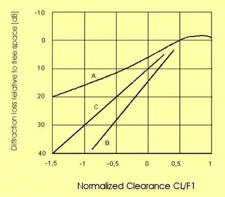
Diffraction Loss vs. Normalized Clearance, with different obstacles: A)
knife edge; B) smooth spherical
earth; C) intermediate
(from ITU-R Rec. P-530, by ITU permission)
![]()
More on
obstruction loss computation
A more
detailed analysis of obstruction loss is reported in ITU-R Rec. P-526, where
general formulas are given. The knife-edge model is also extended to rounded
obstacles and to the case of multiple obstructions.
Knife-edge obstacle - A
good approximation of the obstruction loss produced by a knife-edge obstacle is
given by :
![]()
where ![]() and the
approximation holds for CNORM < 0.5.
and the
approximation holds for CNORM < 0.5.
Single
rounded obstacle - The
obstacle geometry is shown in the figure below, where also the relevant
parameters are graphically defined.
Geometrical parameters in a rounded obstacle
(from ITU-R Rec. P-526, by ITU permission).
An approximate formula for the obstruction loss is :
![]()
where Lknife is given above and DL is the additional loss, compared with a sharp (knife-edge) obstacle, given by:
![]()
The normalized parameters n and r are computed as:
where l is the signal wavelength and the geometrical parameters (d, da, db, R, q) are defined in the figure above.
The approximation holds for :
n > 0 that is for negative clearance (obstacle above the ray trajectory);
r < 1 that, for frequency above 1 GHz, means, in practical terms, that the obstacle should not be very close to one hop terminal.
More complex formulas are proposed in the most recent version (2013) of ITU-R Rec. P.526 (sct. 4.2).
Spherical earth - At frequencies above 1 GHz, the spherical earth formulas give :
![]()
where :
![]()
![]()
![]()
![]()
and finally F is the frequency (GHz), RE is the equivalent earth radius (8500 km for k = 1.33), D is the path length (km), H is the antenna height (m) over the earth surface; Y1, Y2 in the first formula refer to the first and second path terminal, respectively (in the Y formula, use the appropriate antenna height).
Multiple obstacles - Several approximate methods have been suggested to estimate the obstruction loss produced by multiple obstacles in a radio hop. It is to be noted that point-to-point links should be usually designed in such a way to avoid multiple obstacles along the radio path. However, it is useful to have computational techniques to deal also with this problem.
A reliable solution is the so-called Deygout model. Let us consider, at first, a path with two obstacles, as shown below.
Evaluation of two obstacle loss with the Deygout
model
(from ITU-R Rec. P-526, by ITU permission).
First, the clearance is estimated at each obstacle, as if that obstacle is the only obstacle in the path. So, the "most significant obstacle" is identified, as the obstacle producing the worst (most obstructing) clearance (in the example above, this corresponds to point M1).
The overall obstruction loss LTOT is then estimated as :
![]()
where L[XY, YZ, H] is the knife-edge obstruction loss in a radio path from X to Z, where an obstacle is at point Y with height H.
The method can be iteratively extended to more than two obstacles. For the total radio path and then for each "sub-path", the most significant obstacle is identified.
ITU-R Rec. P-526 applies the Deygout model to both knife-edge and rounded obstacles, with introduction of a correction factor (which is negligible when the obstacles are evenly spaced).
Clearance Criteria
We now have all the
elements to establish Clearance Criteria in the design of a radio hop :
· the ray trajectory has been discussed and the minimum k-factor value (most critical condition) has been
assessed;
· the loss produced by path
obstructions has been evaluated as a function of the Normalized Clearance
and using the Fresnel ellipsoid concept.
The Clearance Criteria given by ITU-R (Rec. P-530) are summarized in the figure below. They must be applied both in standard k and in minimum k conditions and take account of different climates and different obstacle shapes.
A chart showing the ITU-R (Rec. P- 530) criteria for path clearance.
The red circle is the Fresnel ellipsoid transversal section,
as seen from one hop terminal, partially obstructed by the ground.
The more stringent criteria for tropical climate are justified by the wider variability in k-factor values observed in those regions.
According to ITU-R, the above rules can be made less tight, in some measure, when frequencies below 2 GHz are used. This means that smaller fractions (by about 30%) of the Fresnel radius can be adopted.
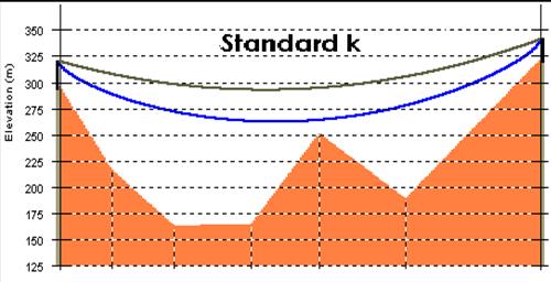
An example of application, with a single isolated obstacle, is given below, in a flat earth representation of the path profile; tropical climate is assumed. First , we check the standard-k condition (100% of the Fresnel ellipsoid free of obstacles). The two lines indicates :
· gray line: ray trajectory (ellipsoid axis) for k = 1.33;
· blue line: lower margin of the Fresnel ellipsoid (100% of the Fresnel
ellipsoid radius).
Then we check the minimum-k condition (60% of the Fresnel ellipsoid free of obstacles). The three lines, in the figure below, indicates :
· gray line: ray trajectory (ellipsoid axis) for k = k min;
· red line: lower margin of the Fresnel ellipsoid (100% of the Fresnel
ellipsoid radius).;
· green line: 60% of the Fresnel ellipsoid radius.
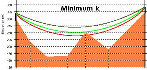
The blue and the green lines, respectively in the two diagrams, are the limiting lines to satisfy the Clearance criteria (the vertical distance from such lines to the ground is usually indicated as the "Margin").
In most cases it is sufficient to indicate those two lines (as derived for k standard and minimum values) on the profile plot and to check that none of them intercepts the path profile (positive Margin).
Further
Readings
Doble J., Introduction to Radio Propagation for Fixed and Mobile Communications (Ch. 1), Artech House Inc., 1996.
Schiavone J.A., "Prediction of positive refractivity gradient for line-of-sight microwave radio path", BSTJ, vol. 60, n. 6, July 1981, pp. 803-822.
Vigants A., "Microwave Radio Obstruction Fading", BSTJ, vol. 60, n.8, August 1981, 785-801.
Schiavone J.A., "Microwave radio meteorology: fading by beam focusing", Int. Conf. Communications, Philadelphia, 1982.
Mojoli L.F., "A new approach to visibility problems in line-of-sight hops", National Telecomm. Conf., Washington, 1979.
End of Session #3
_______________________________________________________________
© 2001-2014, Luigi Moreno,
Torino, Italy