Radio Hop Configuration
© 2001-2014, Luigi Moreno, Torino, Italy
_______________________________________________________________
Summary
In this
Session we introduce the basic configuration of a Point-to-Point Radio Link. The
fundamental parameters useful to describe radio site installations are
presented, including antenna, radio equipment and ancillary subsystems. Hops with passive repeaters are finally
discussed.
Point-to-Point radio-relay links
A Point-to-Point radio-relay link
enables communication between two fixed points, by means of radiowave
transmission and reception. The link
between two terminal radio sites may include a number of intermediate radio
sites.
The direct connection between two
(terminal or intermediate) radio sites is usually referred as a "Radio
Hop". In some cases, a radio hop
may include a passive repeater.
A multi-hop radio-relay link, connecting A to B,
divided in two Radio Sections
A multi-hop radio-relay link can
be divided in a number of "Radio Sections", each of them being made
of one or more radio hops. Transmission
performance are usually summarized on a radio section basis.
General criteria for radio network
planning and design are not discussed here;
just a very brief summary is given below. The overall process can be usually divided in two steps :
1) Preliminary network or link planning. A partial list of
activities carried on at this stage is :
·
Consideration of
Regulatory environment;
·
Identification
of Terminal radio sites;
·
Service and
Capacity requirements;
·
Performance
objectives;
·
Frequency band
selection;
·
Identification
of suitable Radio equipment and Antennas;
·
Sample design
of typical hops, estimate of maximum hop length.
2) Route and Intermediate Site Selection. A number of factors have influence on this choice; among others :
·
Maximum hop
length;
·
Nature of
Terrain and Environment;
·
Site-to-Site
terrain profile; visibility and reflections:
·
Angular offset
from one hop and adjacent hops (to avoid critical interference);
·
Need for
passive repeaters.
·
Availability of
existing structures (buildings, towers);
·
New structures
requirements;
·
Access roads
(impact on installation and maintenance operations);
·
Availability
of Electric Power sources;
·
Weather
conditions (wind, temperature range, snow, ice, etc.);
·
Local
restrictions from regulatory bodies (authorization for new buildings, air
traffic, RF emission in populated areas, etc.);
When a tentative selection of
intermediate sites is available, the final design goes through an iterative
process :
·
Hop
configuration and detailed hop design;
·
Prediction of
Hop and Section performance;
·
Identification
of critical hops;
·
Revision of
Route and Site selection;
·
Revision of Hop
configuration and of detailed hop design.
In the following Sections we focus
on this design process, going through site and hop configuration and leading to
performance predictions. As a first
topic, we discuss the parameters useful to describe the site and hop
configuration.
Site and Hop parameters
A radio hop is described in terms
of :
a) Topographical data and terrain
description :
·
Radio site
position: geographical coordinates or other mapping information; elevation
above sea level (a.s.l.);
·
Path length
and orientation (azimuth: note that in plane geometry the azimuths computed at the two extremes of a
line segment differ by 180 deg, while this is not true in spherical
geometry; so, two path azimuths, referred to each radio site, are usually
indicated);
·
Path profile
as derived from paper or digital maps: note that accuracy requirements are widely
different throughout a radio path, since the elevation of possible obstructions
should be accurately estimated, while significant profile portions (where no
obstruction or reflection is expected) could be almost ignored.
b) Radio equipment, antennas and ancillary sub-systems installed at each
radio site; in the following sections, the main parameters useful to describe
the radio site installation will be discussed.
c) Specific aspects on equipment installation and operation :
·
Antenna
positioning: installation height and pointing; space diversity option, antenna
spacing;
·
Frequency
used: (average) working frequency
(usually referred in hop computations and link budget); detailed frequency plan
(go and return RF channels at each radio site, required for interference
analysis);
·
RF protection
systems (use of 1+1 or n+1 frequency diversity, hot stand-by, etc.)
·
Use of passive
repeaters: flat reflector or back-to-back antenna system, repeater site
parameters, reflector or antenna positioning and pointing.
d) Climatic and environmental parameters: they are usually required by
propagation models (atmospheric refraction, rain, etc.), so they will be
discussed while presenting such models.
Finally, let us consider several
attenuation or degrading factors, such as :
·
Atmospheric
absorption loss;
·
Obstruction
loss;
·
Any other
systematic loss throughout the radio path (additional losses);
·
Rx threshold
degradation due to ground reflections;
· Rx threshold degradation due to interference.
The above impairments will be
discussed in the following sessions, where suitable models to estimate their
impact on hop performance are considered.
However, it may happen that the
inputs required to apply such models are not fully available or that other
reasons suggest not to go through a specific analysis.
In that case, we can include among
hop parameters also a rough estimate (or a worst case assumption) of losses or
degradations caused by the impairments listed above.
Radio Equipment
A
simplified block diagram of a sample radio site installation is shown below.
An example of radio equipment block diagram,
in the case of
multiple RF channel operation, using a single antenna
for both
transmission and reception.
Even if
this example shows a specific configuration, it is useful as a reference in the
following presentation. Other
configurations of particular interest are:
·
Single RF
channel installations, where no branching system is needed;
·
Outdoor
installations, where radio equipment is directly connected to the antenna,
without feeder line.
From the
viewpoint of a single radio hop design, we can limit information about Radio
Equipment to the very basic parameters :
·
Range of
operating frequencies;
·
Transmitted
power PT;
·
Receiver
threshold PRTH (minimum received power required to guarantee a given
performance level);
Note that :
1) Both the transmitted power and
the receiver threshold are usually referred at the equipment input / output flanges, not including branching
filter losses.
2) When the transmitter is
equipped with an Automatic Transmitted Power Control
(ATPC) device, the Tx power to be considered in hop design is the maximum power
level (which should be applied every time the received signal quality is deeply
affected by propagation impairments);
3) The receiver threshold is the
minimum received power required to achieve a given performance level; in
digital systems, the reference performance is usually set at Bit Error Rate
(BER) = 10-3, while other
reference levels may be adopted if needed.
Performance
objectives in digital radio links will be discussed in the final Session of this course.
Additional parameters can be
useful for a more complete understating of the equipment operation, even if
they are not directly involved in the hop design :
·
Equipment user
capacity; for digital systems, bit-per-second or number of standardized signals,
like STM-1 or DS1 signals; for analog
systems, number of telephone or television channels;
·
Bit rate (R)
of the modulated (emitted) signal (this may differ from the user capacity,
mentioned above, since the transmission equipment may include additional bits
for service and monitoring channels, channel coding, etc.);
·
Modulation
technique;
·
Symbol rate of
the modulated (emitted) signal; in analog systems, an equivalent parameter is
the baseband (modulating) signal bandwidth;
·
Emitted
spectrum and modulated signal bandwidth.
The
Symbol rate SR depends on the emitted signal bit rate R and on the
modulation technique :
![]()
where L
is the number of bits coded in a single modulated waveform (L = 2 in QPSK
modulation, L = 6 in 64QAM modulation).
For
advanced tasks in Radio Hop design, more detailed data on radio equipment are
required. This includes :
· Rx noise bandwidth BN and Rx noise figure NF;
· Signal-to-Noise (S/N) ratio at the Rx threshold;
· Co-channel Carrier-to-Interference ratio at receiver input,
producing the threshold BER, in the absence of thermal noise (high Rx level);
· Typical spacing between adjacent RF channel;
·
Net Filter Discrimination (NFD) at the above
spacing;
· Results of signature measurement;
· Possible use of Automatic Transmitted Power Control (ATPC) and
related parameters;
· Possible use of Cross-Polar Interference Canceller (XPIC) and
related parameters.
The Signal-to-Noise (S/N) ratio can be expressed in terms of
received power PR,
receiver noise bandwidth BN, and receiver
noise figure NF :
![]()
where PR is expressed in dBm and BN in MHz; the expression in square brackets gives the receiver thermal noise power.
![]()
Digital
Equipment Signature
The equipment
signature gives a measure of the sensitivity of radio systems to channel
(amplitude and group delay) distortions as produced during multipath propagation events. More specifically, it is used for digital
radio systems with signal bandwidth larger than about 10-12 MHz (on this type
of signals, significant frequency selective distortion is not produced if the
bandwidth is narrower; other signals may be sensitive to frequency selective
multipath even with a narrower bandwidth).
Measurement Set-up
- The Tx signal is modulated by
a test sequence and is transmitted through a simulated multipath channel,
modeled as a two-path channel (direct plus echo branches).
Signature measurement setup.
As
shown in the above figure, the power level and the phase of the delayed signal
can be adjusted by means of a variable attenuator and a variable phase shifter.
Assuming
a normalized signal amplitude equal to 1 in the direct branch and b (< 1) in
the delayed branch, then the Two-Path Channel Transfer Function is:
![]()
t
= Echo delay, assumed as constant ( = 6.3 ns in the original Bell Labs /
Rummler model );
fo
= j / 2 p t = Notch Frequency (corresponding to the minimum
amplitude of the transfer function);
B
= Notch depth (in dB) = - 20 Log10 (1 - b).
Two-path channel transfer
function,
with definition of Notch
Frequency and Notch Depth.
The
above definition refers to a Minimum-Phase Transfer Function. Otherwise, if the signal amplitude is b (
< 1) in the direct branch and 1 in the delayed branch, then similar
definitions apply, but a Non-Minimum-Phase Transfer Function is obtained.
Measurement
Procedure - As shown by the above definitions,
the notch frequency is controlled by varying the echo phase f; while the notch depth depends on
the echo amplitude b.
The
first step in the measurement procedure is to select a given Notch Frequency fo, with echo amplitude close to
zero. Then, the echo amplitude is increased,
making the transmission channel more and more distorting. Consequently, the Bit
Error Rate (BER) will increase.
The
notch is made deeper, up to the "Critical Depth BC", when
BER = 10-3 (or any other desired threshold). The point [BC, fo]
is a signature point.
The same steps are repeated for different
notch frequencies, in order to plot a complete signature curve in the Notch
Depth vs. Notch Frequency plane.
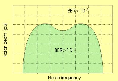
Equipment Signature
in the Notch Depth / Notch
Frequency plane.
In
that plane each point corresponds to a pair of notch parameters, so it is
representative of a particular channel state.
The points below the signature show the channel states for which BER
> Threshold. Therefore, the area
below the signature gives a measure of the receiver sensitivity to multipath
distortions. For an unequalized signal, typical signature width may be of the
order of 1.5 times the symbol rate, while using equalization it is halved at
least.
To
predict multipath
outage, it is often required that the equipment signature be defined by
only two parameters (signature width and depth). In most cases the shape of
actual equipment signatures allow for a "square brick" approximation.
![]()
Equipment
parameters used in Interference analysis
Net Filter
Discrimination (NFD) - It
is used to characterize the radio system ability to limit the interference
coming from an adjacent radio channel.
NFD gives the
improvement in the Signal-to-Interference ratio passing through the Rx
selectivity chain (RF, Intermediate, baseband stages) :
![]()
where (C/I)RF
is defined at the RF input stage and (S/I)DEC at the decision circuit
stage.
Signal spectra at the
receiver input ant output
and Rx selectivity.
As shown by the figure
above, the NFD depends on :
![]() Interfering signal spectrum (Tx filtering);
Interfering signal spectrum (Tx filtering);
![]() Channel spacing;
Channel spacing;
![]() Overall Rx selectivity in the Useful Channel.
Overall Rx selectivity in the Useful Channel.
The NFD can be
measured or evaluated for interference between identical signals (adjacent
channel interference in a homogeneous channel arrangement) and also when the
interfering signal is different (in capacity and/or modulation format) from the
useful one (interference in a mixed signal network).
So, for any pair of
useful and interfering signals and for each value of the channel spacing, a NFD
value can be evaluated.
Threshold
Carrier-to-Interference ratio - In some applications the received signal may be interfered by a
co-channel signal, with identical capacity and modulation format (for example
in co-channel frequency
arrangements, with use of both orthogonal polarizations).
The receiver
sensitivity to co-channel interference is estimated by a Bit Error Rate (BER)
vs. C/I curve, as shown in the figure below.
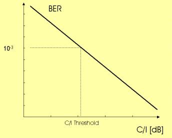
Bit Error Rate (BER) vs.
Carrier-to-Interference ratio (C/I),
with indication of C/I
threshold for BER = 10-3.
The measurement is
made in absence of any significant thermal noise contribution (high Rx power level).
From this measurement,
it is possible to know the Carrier-to-Interference ratio corresponding to the threshold
error rate (for example BER = 10-3).
Cross-Polar
Interference Canceller (XPIC) Gain - The Interference Canceller is used to reduce the interference
coming from a signal transmitted on the same frequency with orthogonal
polarizations (usually the useful and interfering signals have identical
capacity and modulation format).
We assume that the
signal-to-interference ratio at the receiver RF input is (C/I)RF.
The interference
canceller works in such a way that the signal-to-interference ratio appears to
be improved to a higher value (C/I) APP defined as
![]()
where
XPICGain
is defined as the gain produced by the cross-polar canceller. The interference impairment is computed by assuming (C/I) APP to be the actual signal-to-interference
ratio.
Antennas
Gain
definition and related parameters
Let us consider
a radio transmitter with power pT coupled to an Isotropic Antenna (an ideal source of EM Radiation,
that radiates uniformly in all directions). At the distance L from the
antenna, the emitted power will be uniformly distributed on. the surface area of a sphere of radius
L, so that the Power Density rI is :
![]()
EM power emission from an Isotropic Antenna (left)
and from a Directive Antenna (right)
Then we
substitute the Isotropic Antenna with a Directive Antenna, while the
transmitted power is again PT. We imagine to measure the Power Density where the antenna axis
intercepts the sphere surface, with result rD
The antenna gain gives a measure of how much the emitted power is
focused in the measurement direction, compared with the isotropic case. As a result of the "experiment"
described above, the antenna gain is defined as :
![]()
This definition leads to g = 1 for
the isotropic antenna.
Generally
speaking, the antenna gain is related to the ratio between antenna dimension
and the wavelength l. More specifically, in the case of reflector
antennas, the antenna gain g is given by :
![]()
where D is the reflector diameter,
h is called "antenna
efficiency" (typically in the range 0.55 - 0.65), A is the reflector area and
AE = h A is the Antenna Effective Area.(or Aperture).
In logarithmic (decibel) units :
![]()
where the ±0.5 dB term depends again on antenna efficiency; it is assumed to express
the diameter D in meters [m] and the frequency F in GigaHertz [GHz].
Note that, for given dimension,
the antenna gain increases with frequency (6 dB higher if the frequency is
doubled). Similarly, at a given
frequency, the gain increases 6 dB if the antenna diameter is doubled.
Below, some examples of antenna gain vs. diameter and frequency are given.
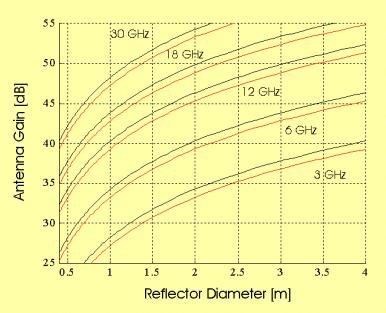
Antenna gain vs. diameter and frequency; the double
(red, black) line gives a range of possible gains, depending on antenna
efficiency.
The 3-dB beamwidth BW (see
graphical definition below) is related to antenna gain; as the gain increases,
the EM energy is focused in a narrower beam.
Definition of the antenna 3-dB Beamwidth BW.
For reflector antennas, some
simple "rules of thumb" are useful in relating antenna diameter D
[m], working frequency F [GHz], gain G [dB], and the 3-dB beamwidth BW [deg] :
![]()
![]()
Note that these are approximate relations, fitting with "real" values within some margin; in particular cases this margin may be even large.
An
additional concept in antenna operation is the Far Field Region. It is the region sufficiently distant from
the antenna, where the electromagnetic (EM) field can be well approximated as a
plane wave and the antenna diagram is stabilized. Closer to the antenna, the
Near Field Region and the Fresnel (transition) Region are defined, where the
antenna radiation diagram is not easily predicted. The boundary between the
Fresnel and the Far Field Region is approximately at the distance :
![]()
Antenna Parameters for hop design
Point-to-point radio hops usually
make use of high-gain directive antennas, which offer several advantages :
· both Transmission and Reception
: the antenna
gain is maximized in the desired direction.
· Transmission : the emitted radio energy is focused toward
the receiver, thus reducing the emission of interfering
radio energy in other directions;
· Reception : the receiver
sensitivity to interfering signals coming from other directions is reduced.
However, in special cases, also
antennas with sectorial or even omnidirectional coverage may be used (this is
true mainly for point-to-multipoint applications).
In most cases, directive antennas
are parabolic antennas or other reflector antennas (like Horn or Cassegrain
antennas). The directivity patterns can
be measured both in the vertical (elevation) and in the horizontal (azimuth)
planes; however, we can often adopt the
simplifying assumption that one diagram is applicable both to the vertical and
to the horizontal planes. In that case, also the 3-dB antenna beamwidth is
assumed to be the same in the two planes.
As far as
interference problems are not considered in a single radio hop design, we can
limit information about the antennas to the very basic parameters :
· Range of operating frequencies;
· Single or Double
Polarization operation;
· Antenna gain;
· 3dB beamwidth in
the vertical plane (this may be useful to analyze reflection paths).
An example of the antenna connection
to radio equipment is given in the Block
diagram shown above. Note that the
antenna gain (as well as other antenna parameters) is referred to the antenna
I/O flange.
Additional parameters can be useful
for a more complete description of antenna operation :
· Antenna type
(Parabolic, Horn, Cassegrain, etc.);;
· Coverage type (omnidirectional, sectorial, directive);
· 3dB beamwidth in
the horizontal plane (for sectorial antennas);
· Diameter (or more
generally, physical dimensions);
· Voltage standing
wave ratio (VSWR);
· Weight.
Moreover, the antenna diagram, as mentioned above, illustrates the antenna operation in directions other than the pointing (max gain) direction.
Antenna radiation diagram (mask) for Co-polar e
X-polar operation
(a different horizontal scale is used in the 0 - 20
deg range and in the 20 - 180 deg range).
![]()
More
on the Antenna radiation diagram
Some additional comments on antenna diagrams :
![]() The result of the
antenna directivity measurement usually exhibits multiple lobes and nulls. A sidelobe envelope is estimated, giving a
"mask diagram", useful to characterize the antenna directivity.
The result of the
antenna directivity measurement usually exhibits multiple lobes and nulls. A sidelobe envelope is estimated, giving a
"mask diagram", useful to characterize the antenna directivity.
In interference analysis the need arises to estimate the
antenna gain in any direction and the antenna mask gives a conservative result.
![]() The pattern of co-pol and
cross-pol antenna diagrams, close to the pointing direction, are significantly
different, as shown in the figure below.
The pattern of co-pol and
cross-pol antenna diagrams, close to the pointing direction, are significantly
different, as shown in the figure below.
Example of Co-pol. and
Cross-Pol. antenna diagrams,
close to the antenna
pointing direction
While the co-pol pattern is
rather flat, in the range of some tens of degree around pointing direction
(maximum gain), the cross-pol pattern has a very narrow minimum in the same
direction.
In some cases it is
convenient to point the antenna by searching for the minimum cross-pol signal level,
instead of searching for the maximum co-pol signal. By this way, it is assured
that, not only the maximum gain, but also the maximum cross-pol discrimination
are obtained.
![]() The antenna
directivity diagram is usually measured in a controlled environment, in order
to characterize the "true" antenna response, without influence or
errors produced by any external element.
The antenna
directivity diagram is usually measured in a controlled environment, in order
to characterize the "true" antenna response, without influence or
errors produced by any external element.
In actual operation, the antenna response may by significantly altered by the surrounding environment. For example, an obstacle close to the main antenna lobe may produce a signal reflection, about 180° from the antenna pointing direction. This apparently reduces the antenna front-to-back decoupling, both in the co-pol and cross-pol diagrams.
The correct antenna positioning is a key factor in order
to get antenna performance in real operating conditions as close as possible to
measured parameters.
Ancillary equipment
A number
of additional equipment and subsystems are working in a radio site. In the
present context, we consider only what is strictly related to the design of a
radio hop (so, we do not discuss power lines and back-ups, air conditioning,
grounding, and other subsystems, even if they are of significant importance in
the overall site operation).
Branching
system
As shown
in the block diagram above, a branching
filter is required in radio transceivers for multiple RF channel operation.
In transmission,
the function of the branching system is to multiplex RF channels on a single
wide-band RF signal, suitable to be transmitted on a single antenna. Similarly, in reception, the branching
system splits the multi-channel signal coming from the antenna into multiple RF
channels, each addressed to the corresponding receiver.
The
branching loss is different for the various RF channels (in Tx and Rx),
depending on the number of filter ports and circulators to be passed through by
the signal. However, in hop design, it
is advisable to take account of highest loss, resulting from Tx and Rx
branching.
In a
branching configuration with a common Tx/Rx antenna (see block diagram), the branching loss include the loss of the
circulator used to separate the Tx and the Rx branches.
Tx /
Rx Attenuators
Power attenuators may be added in the transmitter or in the receiver chain, mainly to avoid an excessive power level at the receiver input (which may saturate the Rx front-end stage) and/or to avoid unnecessary power emission in short hops (interference reduction).
Note that many radio equipments now include power setting options or ATPC (Automatic Transmitted Power Control) devices, so that in most cases the use of external attenuators is no longer required.
In the context of radio hop design, the
only parameter to be associated with Tx and Rx attenuators is the attenuation
level itself.
Feeder
Line
A feeder
line is required to connect the antenna I/O flange to the radio equipment I/O
port (or to the branching system I/O port).
The exception is the outdoor configuration, with direct
equipment-to-antenna connection.
The basic
feeder parameters for radio link design are :
· Range of operating frequencies;
· Specific loss (expressed in dB per
unit length).
Additional parameters, giving more
details on feeder description :
· Feeder type (cable, rectangular waveguide, etc.);
· Weight (expressed in kg per unit length).
![]()
Hops with a Passive Repeater
Passive Repeaters are
used mainly in hops over irregular terrain, to by-pass an obstruction along the
path profile.
Three Passive Repeater
configurations are described below, while the corresponding Link Budget
equations are presented in the next Session.
Single plane
reflector - it
is implemented as a metal surface, which is close to a 100% reflection
efficiency. The surface flatness must be more and more accurate for increasing
frequency (smaller signal wavelength).
The reflector works to
deviate the incoming signal direction by an angle b.
The geometry is shown in the figure below
Passive repeater implemented
as a single plane reflector
Each path from a radio
site to the repeater is called a "leg". So a radio hop with a single reflector is made of two legs.
Note that the useful
or "effective" area AE of the plane reflector is given by
:
![]()
where AREAL
is the real reflector area and j is the angle between the two rays.
It is estimated that
for j > 120° (corresponding to b < 60°) the effective area is
so reduced that it is not practical the use of a single reflector, since very
large panels should be installed.
Double plane
reflector - It
is used when the change in signal direction (b) is lower than 60° or when it is not
possible to find a suitable position for a single reflector, where visibility
with both hop terminals is assured.
Usually, the two
reflectors are arranged fairly close together. A typical double reflector geometry is shown
below.
Passive repeater implemented
as a double plane reflector
A radio hop with a double
reflector is made of three legs.
With a double
reflector arrangement it is possible to operate even if the angle b is close to 0°.
The reflector
effective area is given by the same formula
used for the single reflector, so that the angle between the two rays, at both
reflectors, should be as low as possible.
Back-to-Back
antenna configuration - Another passive repeater arrangement can be obtained by using two
antennas with a short feeder (cable, waveguide)
connection.
Passive repeater implemented
as a two-antenna
back-to-back arrangement
From a geometrical
point of view, the back-to-back antenna system has a wider and more flexible
application field, compared with a single reflector system. From a given repeater position, any change
in signal direction (b)
can be obtained.
However, single or
double reflectors may be implemented, if needed, with surfaces much wider than
the usual antenna size. Moreover, the
reflector efficiency is close to 100%, compared to some 55% antenna efficiency.
So, when the power
budget is limited, the back-to-back antenna system may be a poor solution.
Further Readings
Ferdo Ivanek (editor), Terrestrial Digital Microwave Communications, Artech House Inc., 1989
Anderson H.R., Fixed Broadband Wireless System Design, J. Wiley, 2002.
Lehpamer H., Transmission systems design handbook for wireless networks, Artech House Inc., 2002.
Sun Y., Wireless Communications Circuits and Systems, IEE, 2003.
Doble J., Introduction to Radio Propagation for Fixed and Mobile Communications, Artech House Inc., 1996.
Greenstein, L.l., and Shafi M. (editors), Microwave Digital Radio, Prentice-Hall Inc, 1987.
"Advances in Digital Communications by Radio", IEEE Journal on Selected Areas in Communications, vol. JSAC-5, n. 3, April 1987.
Noguchi T., Daido Y., and Nossek J.A., "Modulation Techniques for Microwave Digital Radio", IEEE Communications Magazine, vol. 24, n. 10, October 1986, pp. 21-30.
Greenstein L.J., "Analysis / simulation study of Cross Polarization Cancellation in Dual-Polar Digital Radio", AT&T Technical J., vol. 64, n. 10, Dec. 1985, pp. 2261-80.
End
of Session #1
_______________________________________________________________
© 2001-2014,
Luigi Moreno, Torino, Italy