Basics in Link Engineering

Summary

Free Space propagation

Terrestrial Radio Links

Link Budget

Fade Margin and Outage Prediction

Link Equation with Passive Repeater

HERALD Lab #2

_______________________________________________________________

Summary

In this Session the Free Space radio link equation is presented, together with the concept of Free Space Loss. Then, terrestrial radio hops are considered and a brief summary is given of the most significant propagation impairments. We discuss the Link Budget, in order to estimate the Fade Margin, and how to use the Fade Margin in predicting the outage probability. Finally, the radio link equation is revised to include the use of passive repeaters.

Free Space propagation

We approach radio link engineering by first considering an ideal propagation environment, where transmission of radio waves from Tx antenna to Rx antenna is free of all objects that might interact in any way with electromagnetic (EM) energy. This assumption is usually referred as "Free Space" propagation.

Let us consider a radio transmitter with power p_T coupled to a directive antenna with maximum gain on the axis g_T.

At distance D from the transmitting antenna (sufficiently large, in order that Far Field conditions are satisfied), the Power Density on the antenna axis is :

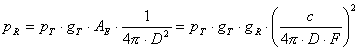
Computation of Received Power in Free Space propagation

Now we imagine that, at the distance D, a receiving antenna is installed. The antenna "effective aperture" or "effective area" A_E gives a measure of the antenna ability to capture a fraction of the radio energy distributed at the receiver location. Assuming no receiver mismatch, the power p_R, at the receiver antenna output flange, is :

Taking account that the relation between the Rx antenna gain and the antenna "effective aperture" is :

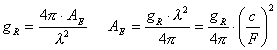
the received power equation becomes :

where F is the frequency of the transmitted signal, l is the wavelength, and c = l F is the propagation speed, which can be assumed to be about 3 10⁸ m/s, with good approximation, both in the vacuum and in the atmosphere.

This is usually known as the "Free Space Radio Link Equation." Using logarithmic units, it can be written as :

where upper-case letters are used to express power in dBm and gains in dB, while the same letters in lower-case had been previously used for non-logarithmic units.

Note that frequency must be expressed in GHz and distance in km, otherwise the 92.44 constant is to be modified accordingly (e.g. : with distance in miles, the constant is 96.57; with frequency in MHz, the constant is 32.44).

The above equation can be also written as :

where FSL is called Free Space Loss, given by:

If we assume to use Isotropic Antennas (G = 0 dB) both at the transmitting and at the receiving site, then :

so FSL is also defined as "loss between isotropic antennas".

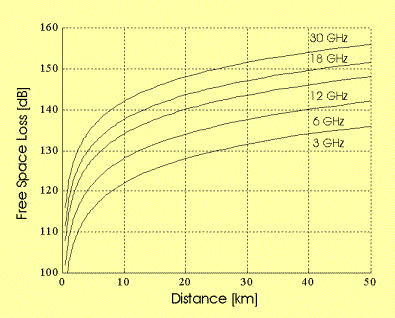
Free Space Loss vs. distance and frequency

Comments on Free Space Loss

The concept of Free Space Loss, and the related formulas, need some comments. First, the term "loss" could suggest some similarity with losses in coaxial cables or other guided transmission of electromagnetic (EM) energy, where we observe an interaction and power transfer from the EM wave to the propagation medium. Here, we are talking about "Free Space Propagation": the propagation medium is the vacuum and no interaction exists. The Free Space Loss is just to be referred to the density of EM energy, which follows the inverse square-law dependence versus distance from the source.

A second problem is the role of frequency in the Free Space Loss formula. Is the Free Space a transmission medium more lossy as frequency increases? Let us consider the two equivalent forms of the radio link equation given above :

The first expression is probably more intuitive and should be preferred when we try to understand the physical concept underlying free space propagation. The Tx antenna is described by its gain (the ability to focus the EM power toward a given direction), while the Rx antenna is described by its equivalent aperture (the ability to capture the EM power distributed at the receiver location).

On the other hand, we passed to the second expression, where both the Tx and Rx antenna gains appear, since it looks attractive for its symmetric form. The frequency dependence in this case is due to the decreasing effective aperture of the receiving antenna (for a given gain), as the frequency increases. It is just a formal artifice to include frequency dependence in the so-called Free Space Loss.

As a conclusion, the Free Space Loss is a convenient step in evaluating the received power in a radio link and it is useful in order to put formulas in a manageable form. However, care should be paid about the physical concept related to it, in order to avoid misleading interpretations.

Terrestrial radio links

We now depart from the Free Space assumption and we put again our feet to the earth. We consider radiowave propagation between two terrestrial radio sites, in the context of radio hop design.

Transmitting and receiving antennas are assumed to be installed on towers / buildings, at moderate height above the earth surface (meters or tens of meters), so that propagation in the lower atmosphere, close to ground, has to be considered.

Moreover, we assume that the radiowave frequency is in the range from UHF band (lower limit 300 MHz) up to some tens of GHz (60 GHz can roughly be the upper limit, according to present applications).

Compared with Free Space Propagation, the presence of the atmosphere and the vicinity of the ground produce a number of phenomena which may severely impact on radiowave propagation.

The major phenomena are due to :

· Atmospheric Refraction :

· Ray Curvature;

· Multipath Propagation;

· Interaction with particles/molecules in the Atmosphere:

· Atmospheric Absorption in the absence of rain;

· Raindrop Absorption and Scattering;

· Effects of the Ground :

· Diffraction through Obstacles;

· Reflections on flat terrain / water surfaces.

When one or more of the above phenomena affect radio propagation, the resulting impairment is :

· usually, an additional loss (with respect to free space) in the received signal power;

· in particular cases, also a distortion of the received signal.

Propagation impairments will be considered in the following sessions. In most cases they can be predicted only on a statistical basis. They are mainly affected by :

· Frequency of operation;

· Hop Length;

· Climatic environment and current meteorological conditions;

· Ground characteristics (terrain profile, obstacles above ground, electrical parameters).

From the viewpoint of the phenomena duration, let us consider :

· temporary impairments, which affect the received signal only for small percentages of time (examples are rain, multipath propagation, ...);

· long-term (or permanent) propagation conditions, which affect the received signal for most of the time (examples are atmospheric oxygen absorption, terrain diffraction, ...), even if their impact may be variable in some measure.

In most cases, long-term propagation impairments do not produce a significant power loss in the received signal, compared with Free Space conditions. So, the received power observed for long periods of time will be rather close to that predicted by the Free Space Radio Link Equation.

The most significant exception to the above condition is experienced in radio paths with not-perfect visibility. In that case, attenuation caused by terrain diffraction results in a systematic loss, in comparison with Free Space conditions.

Link Budget

Even in designing Terrestrial Radio Links, the Free Space Radio Link Equation is the basis for received power prediction.

The equation in logarithmic units offers a very simple and convenient tool, since Gains and Losses, throughout the transmission chain, are added with positive or negative sign, as in a financial budget. The result is what is called the "Link Budget".

The Free Space equation can be re-written with more detail, taking account of actual equipment structure and of systematic impairments throughout the propagation path. An example is given in the Table below .

Power Level [dBm]	Gains [dB]	Losses [dB]
Tx Power at radio eqp. output flange
		Tx branching filter Tx feeder Other Tx losses
Power at ant. input
	Tx antenna gain
		Propagation losses : Free Space Obstruction Atm. Absorption Other
	Rx Antenna gain
Power at ant. output
		Rx feeder Rx branching filter Other Rx losses
Nominal Rx Power at radio eqp.input flange

As shown in the above example, the link budget includes an estimate of the power loss due to permanent (or long-term) impairments (like atmospheric absorption and obstructions). So, the Nominal Rx Power (as computed at the last line) is expected to be observed for long periods of time.

Once the Link Budget is computed, other impairments at the receiver are taken into account as :

· a degrading effect in receiver operation (Rx threshold degradation): this usually applies to the effect of ground reflections and interference;

· a short term attenuation (or even distortion) in the received signal, whose effect may be to fade the received signal below the Rx threshold

Power	Threshold	Margin
Nominal Rx Power
	Equipment Threshold
	Threshold Degrad. Reflections Interference
	Hop Threshold
		Fade margin

We summarize the final steps in Link Budget analysis with the two equations :

Note that Threshold Degradation causes the actual Hop Threshold to be higher than the Equipment Threshold (one dB threshold increase means one dB reduction in the available Fade Margin).

Fade Margin and Outage prediction

Typically, point-to-point radio hops are designed in a way that the Nominal Rx Power (as computed in the Link Budget) is far greater than the receiver threshold. So, rather large Fade Margins (of the order of 30-40 dB, or even greater) are usually available.

The Fade Margin is required to cope with short term attenuation and distortion in the received signal (mainly caused by rain and multipath).

A summary of various definitions is given in the diagram below.

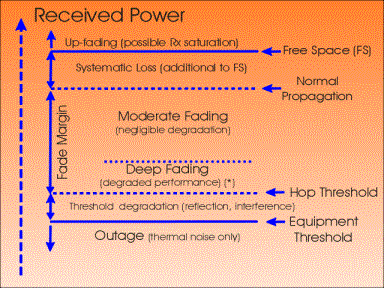
A summary of definitions in Received Power levels, thresholds,

and margins, with application to Outage estimation.

The above figure suggests the following comments :

· The Rx power may exceed the Free Space level: the so-called "up-fading" is a rather unusual event (it may be caused by particular refraction conditions, which create a sort of guided propagation through the atmosphere). Care must be taken that the received power level be in any case below the maximum level accepted by the Rx equipment (otherwise, receiver saturation and nonlinear distortion may be observed).

· The Rx Power will be at the Nominal level (Normal propagation) for most of the time.

· Moderate attenuation below the Nominal Rx power does not usually produce any significant loss in signal quality.

· The Equipment threshold may be degraded in some measure by reflections and/or interference, so that a higher Hop threshold must be considered.

· Starting from the very low Rx power, the Outage conditions are :

· below the Equipment threshold, outage is produced by the receiver thermal noise, even in the absence of any additional impairment in the received signal;

· below the Hop threshold, outage is caused by the combined effect of receiver noise and other impairments (like reflection or interference);

· in the deep fading region, above the Hop threshold, outage may be observed when the received signal is not only attenuated, but also distorted by propagation events (mainly, frequency selective multipath).

From the above discussion, the Outage time, during the observation period To (typically, one month) can be predicted as :

if no contribution to outage is expected from signal distortion.

On the other hand, if significant distortion in the Rx signal is expected to contribute to the total outage, the prediction formula has to be completed as :

where the second term gives the contribution to outage probability when the received signal is above the Hop threshold, but it is severely distorted (note that Prob{A/B} means probability of event A, given that event B is true).

These formulas only help to clarify how the outage time is related to the Rx power level and to additional impairments in the received signal. They do not provide a practical means to predict outage time; this requires that suitable statistical models of propagation impairments be available: Such models will be considered in the following Sessions.

Link Equation with Passive Repeater

When a Passive Repeater is used in a radio hop, we have to revise the "Basic Radio Link Equation".

To be consistent with the simple Free Space formula, we write the new equation as :

where :

FSL(D_TOT) is the Free Space Loss of a radio link with path length D_TOT = S D_i ;

D_i is the length of each path leg;

L_PR is the power loss caused by the passive repeater, in comparison with the Free Space case.

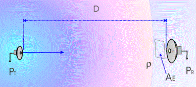
Single Reflector - We refer to the path geometry, as shown in a previous figure and to the definition of the reflector effective area A_E. Then, L_PR is given by :

where F is the working frequency in GHz and D₁, D₂ are the leg lengths in km.

Double Reflector - Again, we refer to the path geometry, as shown in a previous figure and to the definition of the reflector effective area A_E. Then, L_PR is given by :

where F is the working frequency in GHz and D₁, D₂, D₃ are the leg lengths in km.

Back-to-Back antenna system - The path geometry is shown in a previous figure. Then, L_PR is given by :

where F is the working frequency in GHz, D₁, D₂ are the leg lengths in km, G₁, G₂ are the antenna gains at the repeater site (usually G₁ = G₂) and L_F is the loss due to the feeder connecting the two antennas.

Near Field correction - The above formulas are correctly used when the reflectors are positioned outside the "near-field" region. If this condition is not satisfied, then a correction factor (additional loss) must be applied.

The near-field region is estimated as a function of the antenna and reflector dimensions and of the signal frequency (wavelength l). Two normalized parameters (a, b) are computed :

where D_Min is the shortest leg from one antenna to the closest reflector, d is the antenna diameter and A_E is the reflector effective area.

A rule of thumb is the following: for b in the range 0.2 - 1.5 (this covers most practical conditions), the near field correction factor is not negligible if a < (0.5+b). Some examples are given in the Table below :

b = 0.2

b = 0.6

b = 1.0

b = 1.4

a = 0.25

4.6 dB

8.2 dB

9.5 dB

> 10 dB

a = 0.40

1.7 dB

3.9 dB

7.1 dB

9.8 dB

a = 0.60

0.7 dB

1.8 dB

3.8 dB

6.7 dB

a = 1.00

< 0.5 dB

0.7 dB

1.6 dB

3.1 dB

a = 1.50

< 0.5 dB

0.7 dB

1.3 dB